The State of CERES: Updates and Highlights

Introduction

The Clouds and the Earth’s Radiant Energy System (CERES) was initially designed in the late-1980s and early-1990s as a facility instrument for NASA’s Earth Observing System (EOS). Since its inception, NASA’s Langley Research Center (LaRC) has led this effort. CERES has a long history with seven different instruments flying on five different missions since 1997. As of today, six CERES instruments remain in orbit – two are no longer operational: the Proto-Flight Model (PFM) unit flew on the Tropical Rainfall Measuring Mission (TRMM) and functioned for a brief period, and FM2, which was powered-off in January 2025 due to battery constraints on Terra. The active CERES instruments are found on Terra (FM1), Aqua (FM3 and 4), the Suomi National Polar-orbiting Partnership (Suomi NPP) (FM5), and the first Joint Polar Satellite System (JPSS-1) mission, now known as NOAA-20 (FM6). Suomi NPP and the JPSS mission are partnerships between the National Oceanic and Atmospheric Administration (NOAA), which owns the satellites, and NASA, which operates them.

The CERES Team has maintained a history of its Science Team (ST) Meetings, recorded in The Earth Observer. The first CERES STM to be mentioned in the newsletter was the third meeting [Jan. 1990, 2:1, 7], which was listed on the “EOS Calendar.” The earliest full STM summary captured events from the seventh meeting in Fall 1992, CERES Science Team [Jan.–Feb. 1993, 5:1, 11–16]. Since then, the periodic reports (typically spring and fall) have kept readers up to date on the status of the CERES instruments in orbit and the science results from the data gathered. With such a long history of published meeting summaries, it seems fitting that a report on the state of CERES should be among the last articles published by The Earth Observer.

The most recent CERES contribution to The Earth Observer was the article, Update on the State of CERES and Highlights from Recent Science Team Meetings [Sept.–Oct. 2023, 35:5, 43–53]. Since that time, CERES has held four STMs – bringing the total to 42. Norman Loeb [LaRC—CERES Principal Investigator (PI)] hosted all the meetings.

The four most recent meetings were:

• The 39^th CERES STM (Fall 2023) at the NASA Goddard Institute for Space Studies (GISS) in New York, Oct. 17–19, 2023.
• The 40^th CERES STM (Spring 2024) at LaRC in Hampton, VA, May 14–16, 2024.
• The 41^st CERES STM (Fall 2024) at Lawrence Livermore National Laboratory in Livermore, CA, Oct. 1–3, 2024; and
• The 42^nd CERES STM (Spring 2025) at LaRC, May 13–15, 2025.

A Fall 2025 meeting had been scheduled at LaRC from Oct. 28–30, 2025, but was cancelled due to the Federal Government shutdown. Planning is underway for another meeting to be held in Spring 2026.

This article will focus on the Fall 2023 and Spring 2024 meetings – drawing primarily from the State of CERES presentation, programmatic content, and mission and instrument status reports delivered at those meetings. The sections on the State of CERES and Invited Presentations also include content from the Fall 2024 and Spring 2025 meetings. The Contributed Presentations from these latter meetings are not included in this article. For more details the reader is directed to the CERES website where agendas and links to individual presentations can be found for all four meetings.

The content in this article includes updates on the status of the platforms that carry CERES instruments, CERES data products and algorithms, and CERES outreach activities. The remainder of this article will consist of summaries of the invited science presentations given at these meetings, followed by selected science presentations. More information on the topics briefly mentioned in the summary from the meetings is contained in the respective presentations, which are available on the CERES website.

State of CERES

The State of CERES message is a long-standing tradition, opening the CERES STMs. At the beginning of each meeting, Norman Loeb outlined the major objectives of this group, which remained consistent from meeting to meeting. These objectives include host satellite health, instrument calibration updates, algorithm and validation status from the various Working Groups, and progress toward the next CERES reprocessing.

Loeb began the Fall 2023 meeting by reviewing the large increase in global mean surface temperature based on the European Centre for Medium-Range Weather Forecasts Reanalysis (ERA5) model Version 5 (V5) in 2023. The highest anomaly was reported in September 2023 for the period from 1979 to 2023. The CERES absorbed solar radiation (ASR) – a measure of the difference between incoming solar energy and the energy reflected back into space – exceeded the 90% confidence interval anomaly for March through September 2023 except for May, which does not quite exceed it. The net radiation also exceeded the 90% confidence interval through May of 2023. Starting in June 2023, the Outgoing Longwave Radiation (OLR) exceeded negative 90% confidence interval, indicating a release of energy out of the atmosphere; however, the net radiation dropped below the 90% confidence interval for the remainder of the year. The 2023 value even exceeded the 2016 El Niño event. The extremely large ASR and OLR values continued into early 2024.

The CERES Terra FM2 operated in Rotating Azimuth Plane (RAP) mode until it failed in January 2025. After that, Terra FMI switched to RAP mode during Terra’s drifting period. Aqua FM3 likewise operates in RAP mode as Aqua has drifted. This mode allows for capturing data at a larger range of solar zenith angles. For 48 months, the Suomi NPP FM5 has collected rotating-azimuth data; it returned to Cross-track Mode in October 2023. The team noted a small amount of noise periodically detected on the NOAA-20 FM6 shortwave (SW) channel from November 2023 through February 2024. This noise was only observable during space view when the counts approached zero. Several analyses on Earth-viewing footprints could not identify any impact on the SW radiance.

Loeb highlighted some other efforts that are of interest to the group. The World Climate Research Programme (WCRP) started a lighthouse activity on Explaining and Predicting Earth System Change (EPESC) with a focus on understanding and predicting the Earth Energy Imbalance (EEI). This work exemplifies another effort – CERES Model Intercomparison Project (CERESMIP) experiments – that was championed by GISS. The goal is to provide a larger overlap of model output with CERES observations than the earlier Coupled Model Intercomparison Project Phase 6 (CMIP 6), which only observed forcing through 2014 and projected forcing after 2014. Examples of these forcings are Sea Surface Temperature (SST), sea ice concentrations, aerosol and volcanic emissions, and solar irradiance. Climate variability since 2014 is quite pronounced, including EEI, SST trends, Pacific Decadal Oscillation shift, and El Niño events.

During the Fall 2024 meeting, Loeb discussed the impacts of the shifting Terra Mean Local Equatorial Crossing Time. He explained that the SW Top of Atmosphere (ToA) flux difference between NOAA-20 and Terra are smaller in the Northern Hemisphere than the Southern Hemisphere due to closer observation times. The longwave (LW) flux difference is smaller between hemispheres. The CERES team has been collaborating with the European Space Agency’s Earth Cloud, Aerosol and Radiation Explorer (EarthCARE) project to compare results from its Broadband Radiometer (BBR) with those from CERES. Early results showed that EarthCARE’s BBR SW channel is 8% brighter than CERES, and the LW channel is very consistent with CERES – with the possible exception of very cold scenes being colder than CERES. At the May 2025 meeting, Loeb announced that a 25-year Earth Radiation Budget (ERB) record – from March 2000 to February 2025 – has been established.

Bill Smith, Jr. [LaRC] continued the presentation with a review of the progress of the CERES Edition 5 clouds algorithms. This presentation examined the status of balancing the three goals of this effort. He noted the need for consistency between the derived cloud products from the Moderate Resolution Imaging Spectroradiometer (MODIS) on Terra and Aqua and the Visible Infrared Imaging Radiometer Suite (VIIRS) on Suomi NPP and NOAA-20 – especially given the differences in the bands on each instrument. In addition, he discussed the consistency between three generations of geostationary imagers that cover the 25 years in both timeline and across the globe. CERES uses data from NOAA’s Geostationary Operational Environmental Satellites (GOES 9–18); the European Organisation for the Exploitation of Meteorological Satellites’ (EUMETSAT) Operational Meteorological Satellites (Meteosat 5–11); and the Japanese Meteorological Agency’s (JMA) Geostationary Meteorological Satellite (GMS 5), Multifunction Transport Satellite (MTSAT 1R and 2), and Himawari 8 and 9. Finally, Smith presented the accuracy of this approach compared to observations from Cloud-Aerosol Lidar with Orthogonal Polarization (CALIOP) on the Cloud-Aerosol Lidar and Infrared Pathfinder Satellite Observations (CALIPSO) mission.

In his presentations during the Fall 2024 and Spring 2025 meetings, Smith demonstrated improvements with the Edition 5 algorithm showing consistent cloud fraction between MODIS on Aqua and VIIRS on NOAA-20 – with the ocean values being within 2% for both day and night. He noted that additional work still needs to be done for land and polar night. A comparison with CALIPSO data showed that daytime cloud fraction measurements from VIIRS on NOAA-20 are more consistent than those from MODIS on Terra and Aqua. The Edition 5 nighttime algorithm fixes the overestimates in cloud fraction for high clouds, but still underestimates low clouds [below 3 km (1.9 mi)] by 10%. The geostationary imager-derived clouds common three-channel algorithm has better consistency between satellites and day and night cloud fraction. Smith also added that there are some discrepancies in cloud optical depth and particle size between the European Meteosat imager and the other geostationary satellites. The use of the K-D tree algorithm has improved consistency at night with the day cloud properties.

Wying Su [LaRC] explored how fluxes may change if the Angular Distribution Models (ADMs) are created in different weather patterns (i.e. during El Niño and La Niña events). Two sets of Terra CERES ADMs were produced – one using 24 El Niño months and the other using 24 La Niña months. The global differences between SW fluxes composed from these two sets of ADMs were 0.5 Wm^-2 regardless of the period (e.g., El Niño, La Niña, or neutral phase) and showed the same regional difference patterns. Su also explained how to partition the ToA SW fluxes from CERES into visible and near-infrared (NIR) fluxes. She showed how to use spectral radiances generated using look-up tables (LUT) from the MODerate resolution atmospheric TRANsmission (MODTRAN) code and spectral radiances measured by the VIIRS imager to separate the spectrum – see Figure 1. A ratio between the modeled visible band and CERES SW radiance is derived using the LUT. For water clouds, the visible band has the highest albedo due to cloud absorption being near zero. The NIR albedo is much lower than visible band due to high cloud absorption. For ice clouds, the two albedos are closer because ice clouds are more reflective in NIR than the visible band and there is less water vapor absorption above the cloud.

Lusheng Liang [LaRC, Analytical Mechanics Associates (AMA)] discussed the creation of ADMs using additional RAPS data from November 2021 (when Terra started drifting from the Mean Local Time Equatorial crossing of 10:30 AM) to April 2024. This period of observations provided data obtained at a solar zenith angle that is approximately 10° higher in the tropics than was observed during the initial period used for ADM development. New ADMs developed using data from this period have the largest impact for clear sky overland and cloudy sky over ocean versus clear sky over ocean and cloudy sky over land. Liang has also worked to improve the unfiltering coefficients, using the latest version of MODTRAN 5.4, Ping Ying’s cloud properties, two additional view zeniths, seven additional solar zenith bins, and MODIS BRDF kernels over land and snow. The application of these changes to SW and LW from total minus SW resulted in a -0.30 and 0.30 W/m² respectively for July 2019. Since NOAA-20’s FM-6 instrument has a LW channel, the team made an effort to reduce the differences between the LW channel from the total channel minus the SW channel. They also created a correction using warmer temperatures for the model over desert areas and cooler temperatures over vegetated land.

Dave Doelling [LaRC] presented a method to compare data from two ERB instruments in the same orbit, such as CERES on NOAA-20 and Libera on JPSS-4. This method is necessary without data from Terra. This approach used the invariant target of Libya-4. He compared the results using CERES instruments on Suomi NPP and NOAA-20. He added a second target to this analysis: Deep Convective Clouds that have cloud tops below 220 K located in the Tropical Western Pacific. Another approach placed the CERES instrument in a scan mode, matching the view zenith of the geostationary orbiting satellites (i.e., Terra FM2, Aqua FM3, and METSAT-11). The geostationary imager radiances were used to determine the broadband LW flux, which was compared to the CERES-observed LW flux. The regression of these matched pairs of radiances showed that the Terra and Aqua CERES LW regression are within 0.2%. A machine learning approach to determine LW broadband flux from geostationary satellite imager radiance data showed a 75% decrease in bias and a 9% decrease in Root Mean Square Error over the multi-linear regression approach used in Edition 4. Doelling used a similar approach when working with data from the VIIRS imager, using radiance measurements to assign LW and SW fluxes to the cloud layers in the CERES footprint. When normalizing the individual portion of the footprint to the observed CERES data, the global bias is less than 1 W/m².

In the Spring 2025 meeting, Doelling reported on the small change in monthly global variables from using MERRA-2 instead of GEOS 5.4.1 reanalysis in production of the Single Scanner Footprint (SSF) one degree and Synoptic one degree based on a minimum of a year overlap. He also highlighted the changes in the next version of SYN1deg Edition 4B. These changes included reprocessing of the three two-channel satellites (GMS-5, Met-5, and Met-7), using interpolated cloud retrievals over twilight hours (solar zenith > 60 degree), and transition to using data from NOAA-20 only and MERRA-2 reanalysis after March 2022.

Seung-Hee Ham [Analytical Mechanics Associates/LaRC] reported the availability of instantaneous Terra and Aqua CERES computed fluxes at the surface and ToA on a 1° equal angle grid [CERES Cloud and Radiative Swath (CRS1deg-Hour)] from January 2018 to December 2022. The algorithm changes to the Edition 5 Fu-Liou radiative transfer calculations reduced the LW ToA flux bias to less than 0.5 W/m² from around 2 W/m² with Edition 4.

Ham also discussed plans to increase the number of bands (from 18 to 29) in the Fu-Liou radiative transfer calculations and the corresponding shift in wavelength cut-off used for the bands. Nine gas species will now be used in Edition 5 for each band instead of the maximum of four species used in only one band currently. The line-by-line gas database has also been updated. These changes have less than a 2 W/m² change in the SW and LW broadband fluxes between Edition 4 and 5, but line-by-line results show better performance.

Seiji Kato [LaRC] evaluated the computed irradiance trends at the ToA, surface, and within the atmosphere. At ToA for all-sky conditions, SW flux has been increasingly adding energy. Conversely, LW flux has been removing the additional energy, but at a smaller rate leading to an overall increase in net energy. At the surface for all-sky conditions, SW flux has been increasing energy, while LW flux has been decreasing at almost the same rate. As a result, there has been a small net increase. Within the atmosphere, the SW flux has increased more than the LW flux, but they are both positive. The global all-sky mean aerosol direct radiative effect from the synoptic one-degree (SYN1deg) was -2.2 W/m², which was just below the -2.0 W/m² mean from previous studies.

Paul Stackhouse [LaRC] presented the impact of transitioning the meteorology used in Fast Longwave and SHortwave Flux (FLASHFlux) to the Goddard Earth Observing System–for Instrument Teams (GEOS-IT) product. The global mean difference was less than 0.5 W/m² in LW daytime surface downward flux, but the zonal bias can reach an absolute value of 5 W/m² – see Figure 2.

The Global Learning and Observation to benefit the Environment (GLOBE) clouds team ran Eclipse Challenges during the October 2023 annular and April 2024 total solar eclipses. During each event, citizen scientists were encouraged to collect temperature and clouds measurements before and after the eclipse. The participants collected 34,000 air temperature measurements (which is 2.3 times the average number of observations) and 10,000 (13 times average) cloud measurements for both events. The cloud data showed a decrease in cloudiness as the eclipse approached and an increase after, but contrails showed a steady increase. The data also showed a noticeable decrease in air temperature at the local eclipse maximum.

Invited Science Presentations

The CERES STM typically invites two presentations at each meeting. The summaries for these presentations appear here in chronological order. The Fall 2023 presenters looked at responses to greenhouse gas (GHG) radiative forcing. The Spring 2024 presenters explored the Earth’s hemispheric albedo symmetry and the impact of aerosol changes on the cloud radiative effect (CRE). The Fall 2024 presenters discussed preparation of forcing datasets for CMIP 7 and cloud feedback in models. The Spring 2025 presenters explored trends in spectral radiances and the radiative forcing pattern effect.

Ryan Kramer [NOAA, Geophysical Fluid Dynamics Laboratory] explored the decomposition of the EEI as a tool for monitoring climate change. Kramer explained a Making Earth Systems Data Records for Use in Research Environments (MEaSURE) effort to pull together records from multi-instruments needed for decomposition of radiation forcing and radiative feedback from temperature, water vapor, ToA flux, surface albedo, and CRE – see Figure 3. The portion of the total radiative imbalance not attributed to feedback is due to radiative forcing from LW flux, 0.27 W/m². This result – supported by observations and by results from the Suite of Community Radiative Transfer codes based on Edwards and Slingo (SOCRATES) – used a radiation scheme created by researchers at the United Kingdom Meteorological (UKMet) Office, where the radiative forcing is caused by an increase in GHG. The atmospheric cooling is balanced with sensible and latent heat flux related to precipitation. Latent heating from precipitation is inversely correlated with atmospheric radiative change. Decomposed atmosphere radiative forcing and feedback showed how GHGs radiatively heat the atmosphere but mute the trend in global precipitation. The reduction of aerosol in China since the 2008 Summer Olympics has regionally increased the SW radiative forcing. This result provides an example of the impact of mitigation efforts. GHG forcing is stronger in the tropics due to larger concentrations of water vapor and decreases in extratropical regions.

Susanne Bauer [GISS] examined aerosol and cloud forcing in relation to GHG forcing. Early in the twentieth century, data show aerosols counterbalanced 80% of the GHG forcing, but aerosols began to decrease at the start of this century, reducing their impact to 15% today. The direct aerosol forcing follows the mean aerosol optical depth. It reached the maximum impact in 1977 but has decreased slightly since then. The indirect aerosol forcing is four times larger than the direct forcing and reached its peak in 2007. GISS model version E.21 underpredicted the SW ToA trend and overpredicted the LW ToA – see Figure 4. The version E.3 model received a major upgrade in model physics, cloud microphysics, and turbulence scheme, resulting in substantial improvement modeling marine cirrus clouds, total cloud cover, and precipitable water vapor. The trend in LW ToA flux matches CERES in non-polar regions. While the SW all-sky trend shows improvement, it still underpredicts observations. For example, model aerosol is not picking up the biomass burning in Siberia, which seems to be an artifact of using an older emission data base for the study. The improved aerosol data results reveal a larger trend in cloud droplet number concentration compared to the observations gathered by the Terra satellite. These data remain consistent with the Precipitable Water Vapor trend.

Michael Diamond [Florida State University] discussed a proposed test to evaluate whether Earth’s hemispheric albedo symmetry can be maintained. Currently, the all-sky albedo is nearly equal in both hemispheres, but the ToA clear-sky albedo is much greater in the Northern Hemisphere than the Southern Hemisphere, due to the distribution of landmasses. The Southern Hemisphere is also brighter in the visible wavelength, but darker in near-infrared spectrum. This symmetry is unique.

If the Earth was arbitrarily broken up into hemispheres, less than one-third of these hemispheres would be balanced within 1 W/m². The solar reflection is symmetric, but outgoing LW radiation is not – with less energy leaving the Southern Hemisphere. This global imbalance is reduced with interhemispheric transport through the ocean and atmosphere.

Diamond discussed potential physical mechanisms that could maintain this symmetry (e.g., cloud feedback, solar climate intervention, or hydrological cycles). He noted that surface aerosols and high clouds increase albedo in the Northern Hemisphere, whereas low and altostratus clouds increase albedo in the Southern Hemisphere. Earth’s strong hemispheric albedo asymmetry is transient, which should allow for “natural experiments” to test the mechanism to maintain the symmetry. He discussed the moderate but long-term test for the loss of Arctic sea ice from 2002 to 2012, as well as the decline in clear-sky atmospheric reflection due to air pollution over China that peaked in 2010 and declined in 2019. He also discussed more abrupt changes, including the post-2016 decline in Antarctic sea ice, the decrease in Northern Hemisphere low cloud reflection caused by sulfur fuel regulation as enacted by the International Maritime Organization in 2020, the decreased Northern Hemisphere aerosol concentration following activity restrictions during the COVID-19 pandemic, the increased Southern Hemisphere aerosol concentration during the bushfires in Australia between 2019 and 2020, and the increased Northern Hemisphere aerosol concentration reflection following the Nabro volcanic eruption in 2011 – see Figure 5. Despite these multiple events, the expected change in clear-sky albedo from the surface or aerosol change seems to be masked in the all-sky albedo through simultaneous changes in cloud reflectivity. Many of these events overlap, which complicates how to interpret the results.

Daniel McCoy [University of Wyoming] discussed his investigation of uncertainty in cloud radiative feedback in climate forcing due to changes in aerosols. At this time, extratropical cloud feedback has an uncertainty of over 2.5 W/m². Pollution leads to an increase in aerosol concentration, which impacts cloud formation and changes the droplet number concentration. This increase results in changes to the cloud coverage and amount of liquid water content in the clouds – see Figure 6. The work of McCoy and his colleagues has constrained the change in droplet number and liquid water content with the hope of narrowing the effective radiative forcing from aerosol–cloud interaction. Using results from the Community Atmosphere Model (CAM) 6 and observations, they were able to constrain the range of possible droplet number concentration by 27% and liquid water content by 28%. These constraints reduced the effective radiation forcing to 2%. McCoy argued that this small impact is due to the interaction between precipitation efficiency and radiative susceptibility through changes in the Liquid Water Path (LWP), which results in buffering of the radiative effect by reduced radiative sensitivity.

David Paynter [Geophysical Fluid Dynamics Laboratory (GFDL)] explored the spectral dimension of recent changes in ERB. The atmospheric state, temperature, and gas species, from each level in a grid box are used in a line-by-line (LBL) radiative code to calculate the spectra. The two codes used are the NOAA GFDL GPU-enabled Radiative Transfer (GRT) and the Reference Forward Model (RFM) from Oxford University. Paynter and colleagues used a LW radiation solver to get ToA fluxes. They then compared the monthly mean spectrally resolved ToA fluxes using ERA5 inputs for 2003 to 2021 to Atmospheric Infrared Sounder (AIRS) observations. Paynter showed that there is generally good agreement between all-sky AIRS climatology and the LBL calculations, and similar spectral trends; however, some bands have larger differences in the trend. The all-sky OLR between the LBL-ERA5, CERES, and AIRS show consistent positive trends between 0.15 to 0.31 W/(m²/decade); however, the LBL-ERA5 0.11 W/(m²/decade) and the CERES -0.15 W/(m²/decade) show disagreement.

David Thompson [Colorado State University/University of East Anglia] studied the pattern associated with ToA radiative response to changes in surface temperature. Historically, this has been accomplished by looking at the local radiative response due to local change in temperature or to global-mean temperature change. The first reflects a two-way interaction between the local radiative flux and local temperature that identifies areas that are changing. The second results are more difficult to interpret because the local response is multiplied by the same value. Thus, Thompson proposed a third method of evaluating the changes by using the global-mean radiative response to changes due to local changes in temperature. This approach identifies positive values with warm temperatures and downward radiative fluxes. The temperature variability over the Eastern Tropical Pacific contributes to positive values in the global internal feedback parameter. The reverse happens in the Western Tropical Pacific. Another advantage of this method is that the contribution of local feedback to the global feedback is easy to calculate. Using the CERES monthly-mean Energy Balanced and Filled (EBAF) data, the global weighted feedback is -1.1 W/m² with global oceans contributing -0.2 W/m² and global land -0.9 W/m². The Eastern Tropical Pacific contribution is 0.1 W/m² and the Western Tropical Pacific contribution is -0.1 W/m². This approach can be applied to models to see which are representative of the observations. Preindustrial runs of the model generally reproduce the negative Western Tropical Pacific anomaly; however, Thompson noted that most models do not capture the positive anomaly in the Eastern Tropical Pacific.

Contributed Science Presentation

The following section provides highlights from the contributed science presentations. The content is grouped by Earth radiation instruments that are in development; new techniques for use in climate models and analysis of their results; applications of machine learning; and observational datasets and their analysis.

Future Earth Radiation Instruments

It should be noted that the information shared below reflects the mission plans at the time of the meeting. The mission goals may have changed as a result of changing budgets, agency priorities, and other factors.

Kory Priestly [LaRC] discussed the Athena Economical Payload Integration (EPIC) pathfinder mission using the NovaWurks Hyper Integrated Satlet small satellite platform that is integrated with a spare CERES LW detector and calibration module flight hardware. This setup was designed to test the novel building block approach to satellites as a potential path for the next ERB instrument at a reduced cost. [UPDATE: The Athena mission launched successfully on July 23, 2025. Unfortunately, after being released from the rocket the spacecraft started tumbling and could not be recovered.]

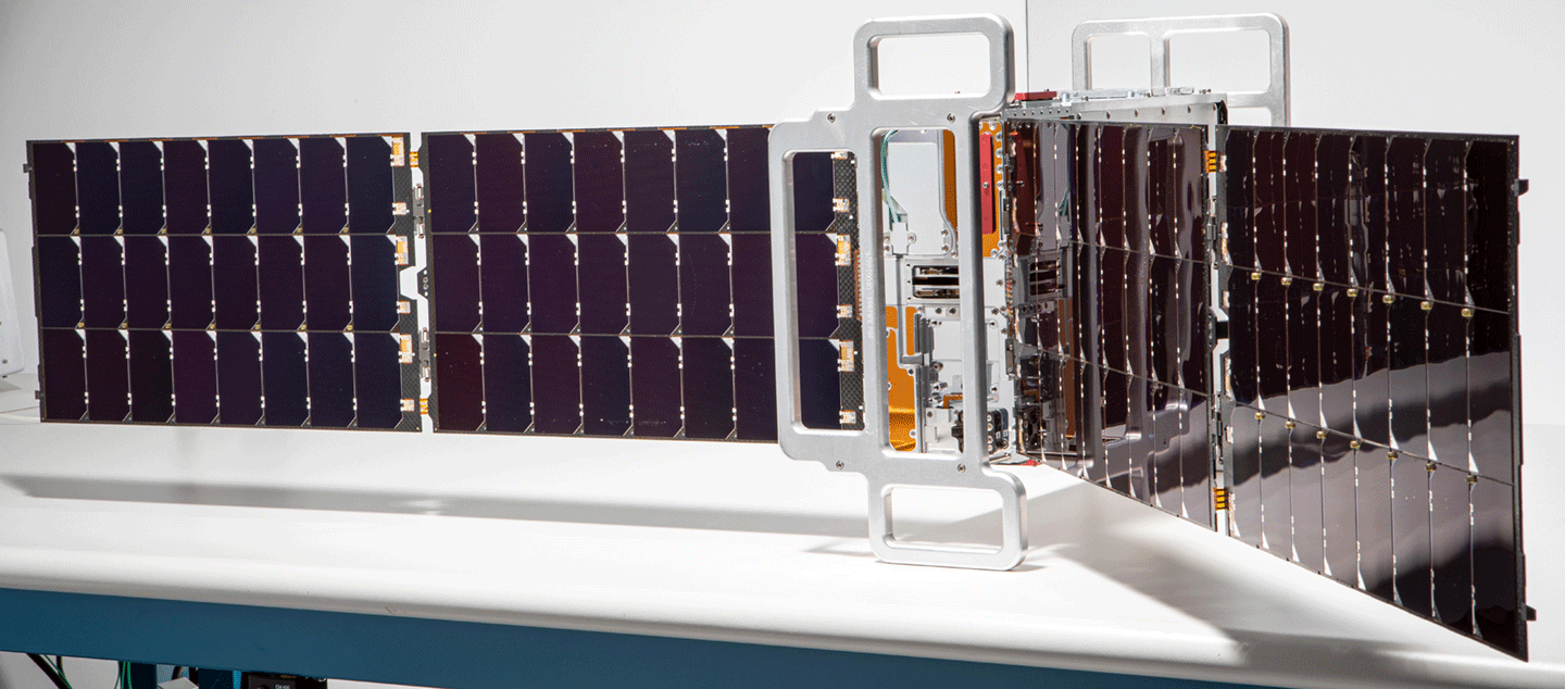
Tristan L’Ecuyer [University of Wisconsin–Madison] presented the science being answered by the Polar Radiant Energy in the Far InfraRed Experiment (PREFIRE) – see Photo 1. The instrument will quantify the far-infrared spectrum beyond 15 mm, which accounts for over 50% of the OLR in polar regions. Additionally, the atmospheric greenhouse effect is sensitive to thin clouds and small water vapor concentration that have strong far infrared signatures. PREFIRE consists of two CubeSats in near polar orbits. The instrument has a miniaturized infrared spectrometer covering 5 to 53 mm with 0.84 mm sampling and an operational life of one year. A complete infrared emission spectrum will provide fingerprints to differentiate between several important feedback processes (e.g., cloudiness and water vapor) that leads to Arctic warming, sea ice loss, ice sheet melt, and sea level rise. [UPDATE: The two PREFIRE CubeSats launched successfully in May and June of 2024, with first light images following in September 2024; public release of PREFIRE data products occurred in June 2025.]

Peter Pilewskie [Laboratory for Atmospheric and Space Physics (LASP)] announced that Libera will be integrated on Joint Polar Satellite System-4 (JPSS-4), which eliminates the need to remove JPSS-3 from storage. This change will affect the launch order. He also presented a comparison between the Compact Total Irradiance Monitor (CTIM) CubeSat and CERES observations. Pilewskie noted that CTIM uses the same Vertically Aligned Carbon Nanotube (VACANT) detectors that Libera will use. Even though CTIM is designed to measure Total Solar Irradiance, the spacecraft has been oriented to get Earth views during spacecraft eclipse with the Sun (nighttime). CTIM provides a ~170-km (105-mi) footprint – which is about eight times larger than that of CERES. The mean relative difference between CERES and CTIM matches are -1.8% varying between -1.5% for FM6 and 2.0% for FM1.

Climate Model Developments and Analysis

Paulina Czarnecki [Columbia University] introduced a method to use a small number of wavelengths to determine broad band radiative fluxes and heating rates as an alternative to the correlated K parameterization approach. It uses a simple optimization algorithm and a linear model to achieve accuracy similar to correlated K-distribution. The approach uses a small set of spectral points – 16 in the study – to predict the vertically resolved net flux within 1 W/m² under clear-sky conditions.

Sean Cohen [Columbia University] addressed the impact of rising surface temperature on precipitation. This information is required to determine the relationship between hydrological sensitivity and radiative cooling sensitivity, where convective heating is balanced by radiative cooling. When carbon dioxide (CO₂) increases, it masks changes in emission from water vapor, resulting in mean rainfall changes when atmospheric transmission changes at a rate of 2%/K. The “symmetry” of the water vapor spectral window causes atmospheric transmission to change at a near constant rate with the surface temperature. This hydrological sensitivity peaks at subtropical surface temperatures – see Figure 7.

George Tselioudis [GISS] explored how shifts in the atmospheric zonal mean circulation changed the CRE. The poleward shift in the location of the Hadley Cell (with corresponding high clouds following it) occurred in both hemispheres; however, it produced SW CRE warming during North Atlantic winter, contrary to SW CRE cooling in both Southern Hemisphere summer and winter. The Southern Hemisphere high cloud shift does not reduce the total cloud amount that occurred in the North Atlantic. The jet stream shift only had an impact during North Atlantic winter. The LW CRE produced a dipole of warming at the previous and new Hadley Circulation positions. The magnitude of LW CRE changes increased with larger upward velocity changes. The SW CRE is dependent on both change in vertical velocity and stability (EIS). Based on these observational findings, Tselioudis evaluated the CMIP 5 and 6 results. Both model results showed lower midlatitude SW CRE warming, but CMIP 5 produced a larger dependence on the climatological Hadley circulation whereas CMIP 6 did not. CMIP 6 models are less dependent on vertical velocity than the earlier set, which allow them to produce Southern Hemisphere SW CRE warming.

Gregory Cesana [GISS] investigated the tropical stratocumulus and shallow cumulus SW feedback, which explains part of the spread in climate sensitivity in the CMIP 5 and 6 models. Observationally, inferred low-cloud feedback is driven by stratocumulus clouds with very little input from cumulus clouds. In the model, cloud type is determined from the mean low cloud fraction in the tropics. When the model cloud fraction is smaller, the cloud is assumed to be cumulus. When it is greater, the cloud is considered to be stratocumulus. CMIP 6 underestimates both low cloud types, but especially in the high stratocumulus regions along the western coasts of continents. Both models favor cumulus over stratocumulus regimes, but the bias for CMIP 6 is less than CMIP 5. The increased model stratocumulus is correlated with increased low-cloud feedback – see Figure 8. If the increased stratocumulus clouds in CMIP 6 matched observations, the mean low cloud feedback would have doubled to 0.7 W/m² K.

Patrick Taylor [LaRC] explored the cloud–sea ice feedback mechanism – see Photo 2. He explained that results from CMIP 5 and 6 show the largest variation in climate projections in the Arctic – where surface albedo feedback is the biggest contribution to the inter-model differences. He evaluated the difference between ice-free and ice surfaces on either side of the marginal ice zone – a part of the seasonal ice zone ranging from 100- to 200-km (62- to 124-mi) wide that extends from the ice edge into the ice pack. The cloud property differences are strongly tied to the differences in thermodynamic profiles, whereas the ice edge (part that is over open water) has warmer, moister, and weaker lower tropospheric stability than the ice pack, leading to more positive turbulent surface fluxes at the ice edge. The feedback from surface properties and lower tropospheric thermodynamics profile are critical to sea ice loss. This sea ice–cloud feedback is positive in the fall and winter and negative in the spring.

Doyeon Kim [LaRC—NASA Postdoctoral Program] discussed factors that explain the current Arctic albedo and possible future changes in this region. She noted that the Arctic undergoes rapid warming during the summer with an accompanying decrease in surface albedo each year until it starts to increase again in the fall – see Figure 9. Researchers use the output from the Atmospheric Model Intercomparison Project (AMIP) and CMIP 6 to infer future changes to albedo. In her analysis, Kim decomposed surface albedo into five terms: sea ice albedo in ice region, sea ice concentration, albedo spatial variation, ice region, and albedo in ocean region. She explained that the ice albedo term drives most changes in AMIP where the ice concentration is held constant. Sea ice concentration and ice region terms become important for the CMIP 6 model where they can change.

Kim went on to look at the monthly averages of albedo, pointing out that March and September show large differences. The multimodal mean exhibits a large spread in the ice albedo. The CMIP 6 spread is significantly influenced by both seasonal and spatial variations. During the early summer months, the ice region term contributes to albedo spread across the Barents, Kara, and Laptev Seas and Greenland Sea. The ice albedo term during the late summer contributes to albedo in the East Siberian, Chukchi, and Beaufort Seas and Central Arctic Sea. A significant inter-model spread may be the primary factor that is contributing to the variability observed in Arctic warming across the different model simulations. Kim discussed the significant difference in surface albedo between CERES and the CMIP 6 models. Both ice fraction and ice albedo have a substantial effect on the model spread of albedo. Time series data indicate that sea ice albedo and concentration remain relatively unchanged in response to global warming while the ice region term decreases significantly.

Application of Machine Learning

Ben Scarino [LaRC, Analytical Mechanics Association (AMA)] explored the consistency of skin temperature (i.e., temperature at the surface) and the temperature 2-m (6.5-ft) above the ground from reanalysis and satellite and ground observations, respectively. He reported that the Global Modeling and Assimilation Office (GMAO) does not assimilate either skin or ground temperature into their reanalysis, producing large biases in those values. Conversely, ERA5 does assimilate 2-m temperature in the reanalysis, which reduce variations by 1 K. The introduction of a Deep Neural Network (DNN) adjusts the reanalysis skin temperature to the observed satellite skin temperature – see Figure 10.

Sunny Sun-Mack [LaRC, AMA] described her efforts to train a Neural Network to identify single and multilayer ice-over-water and cloud top height using the Cloud Aerosol Lidar with Infrared Pathfinder Satellite Observations (CALIPSO), CloudSat, and MODIS [CCCM] pixel-level product from 2008. For single layer cloud top heights, the neural network reduced the standard deviation of difference by nearly half. For the ice cloud top height in multilayer clouds, the standard deviation of difference is one-third. The neural network showed the same “skill” with lower multilayer cloud top heights as it did with single and multilayer upper cloud top heights – (e.g., standard deviation of difference is similar). The single layer cloud base showed similar skill to cloud top height, but the upper cloud base height was slightly worse than the cloud top height. The current algorithm using only imager data cannot differentiate multilayer clouds and creates a single water cloud that does not allow the flux to be calculated properly.

Jay Garg [LaRC/ADNET Systems, Inc] described improvements in SW surface flux using a Machine Learning technique over parameterized instantaneous CERES footprint fluxes. He trained a Neural Network model using the Fu-Liou calculated CERES CRS surface fluxes. This approach reduced the bias from 25 Wm^-2 to almost 0 and the Root Mean Square (RMS) Error from nearly 100 to 13 W/m² for SW surface fluxes. The LW flux statistics showed the bias reduced from 2 Wm^-2 to nearly 0 and RMS Error from 12 to 3.5 W/m² compared to the parameterized flux. These results nearly match the CRS values. Garg explained the plan to implement the Neural Network in the FLASHFlux SSF product – see Figure 11.

Takmeng Wong [LaRC] presented recent progress on an imager independent instantaneous flux product to replace the current Earth Radiation Budget Experiment (ERBE)-like product. Wong described the use of a Random Forest classification technique to determine if the scene is clear (defined as 99.9% cloud free) or cloudy. This approach allowed the CERES radiances to be unfiltered – see Figure 12. Wong and colleagues developed separate models for day and night as well as for surface types (e.g., water, land, desert, and ice and snow). Wong discussed how an Artificial Neural Network was used to convert radiances to a flux. Similar to the radiance models, Wong and colleagues did separate analyses for day and night and for the four surface types for both clear and cloudy conditions. The results from this approach were shown superior to the ERBE-like fluxes but not reaching the accuracy of the SSF using imager-derived clouds.

Eshkol Eytan [University of Colorado, Boulder] focused his work on the cloud twilight zone, an area of transition between clear and cloudy skies, such as cloud halo, cloud fragment, and thin clouds only seen in forward scatter. The clear sky reflectance increases, which is wavelength dependent the closer it is to the cloud. Eytan looked for this feature in the LW data. The lower bound for low clouds is ~0.75 W/m². The fraction of what is considered clear is 60% cloudiness. The cloud twilight zone contribution to the CRE is ~0.8 W/m² for warm clouds and ~8 W/m² for all clouds. Eytan broke down MODIS data into 200-km² (77-mi²) regions and applied a cloud mask. The team then looked at how different channels react with distance. Eytan and colleagues analyzed both visible and LW channels on MODIS. This work determined a pure clear sky value based on distance from known clouds and how it differs from the individual pixel radiance squared divided by the standard deviation obtained in the box. When the twilight spectral measure is greater than one, it signifies cloud contamination. The pure clear MODIS pixels within a CERES footprint are averaged to get a true clear-sky radiance. Often a CERES footprint exceeds the pure clear area. Eytan then explained how he used the clear sky measurement to determine a normalized factor for MODIS data to estimate CRE. He used machine learning between CERES radiances and MODIS radiances at different wavelengths to get pure clear-sky fluxes in homogenous areas. After training on CERES footprint, he then applied MODIS data to smaller areas. The shift of CRE to a higher value, from -6 W/m² to -10 W/m² with imager pixels, produced a more confident cloud mask – reducing uncertainty by a third. This value is still larger than the estimated aerosol direct radiative field. Applying the same technique to the thermal portion of the CRE is 1 and 1.5 W/m².

Observational Datasets and Analysis

Lazaros Oreopoulos [GSFC] presented a new approach for classifying cloudiness at monthly time scales that preserves some of the variability of the original MODIS daily pixel observations. Starting from the 12 previously defined MODIS cloud regimes (CRs) that classified cloud mixtures according to how cloud top pressure and optical depth co-vary on daily scales, he grouped mixtures of CRs occurring regionally over a month using k-means clustering. He classified the geographical distribution of mean occurrences of the resulting eight monthly climatological cloud regimes as “Regimes of Regimes” (RORs) – see Figure 13. When examining the CRE of the RORs, he found that ROR5 contained large amounts of shallow convection. CR10 exhibited strong shortwave and longwave CRE trends because of declining CR10 populations.

Maria Hakuba [NASA/Jet Propulsion Laboratory (JPL)] provided an update on the WCRP Global Energy and Water Exchanges (GEWEX) Data and Analysis Panel assessment of the EEI. Quality control led to a skew in the Ocean Heat Content estimates, mapping techniques, and mask and coverage. The year-to-year variability did not follow the CERES EEI; however, a combination of in-situ and altimetry data for hybrid estimates resulted in very good agreement. The agreement with the JPL geodetic ocean heat uptake with the correct expansion efficiency was also good. The net all-sky was positive across all zones. The net clear-sky trend matched all-sky. The net-CRE showed negative trends in Northern Hemisphere deep tropics and high latitudes. The SW and LW CRE complement each other both globally and zonally. The positive SW CRE dominated in the tropics with fewer, lower, and thinner clouds.

Jake Gristley [NOAA’s Cooperative Institute for Research in Environmental Science (CIRES)/University of Colorado, Boulder] explored the angular dimension of ERB with the Wide Field of View camera planned for the Libera mission. The camera is a 2048 x 2048-pixel array that samples the entire Earth disk subtended from the satellite. It provides 1-km (0.62-mi) pixel spacing at nadir with a single spectral channel at 555 nm. This technique produces more data than can be downloaded. The ADM sampling methods Gristley used encompass the Libera Point Spread Function and minimize the amount of data that must be transmitted.

Seung-Hee Ham discussed how to evaluate cloud volumes using CALIPSO, CloudSat, and MODIS observations separately and in combination to determine the strengths and weakness of each approach. CloudSat misses thin cirrus and low clouds; CALIPSO misses low and mid clouds as a result of signal attenuation; and MODIS misses high and low clouds and over detects mid clouds. Ham described a trend from 2008 to 2017 that shows an increase in the upper-most clouds and a decrease in underlying clouds. She also looked at the El Niño Southern Oscillation (ENSO) signal that showed varying responses based on latitude bands. The increase in high clouds above 10 km (6.2 mi) represent an increase in clouds with a temperature between 220 and 240 K. The colder cloud emission and smaller OLR provide positive cloud feedback.

Brent Roberts [NASA’s Marshall Space Flight Center (MSFC)] presented applications of CERES surface fluxes in the Regional Visualization and Monitoring System (in French SERVIR). SERVIR is a joint initiative of NASA, United States Agency for International Development (USAID), and leading geospatial organizations in Asia, Africa, and Latin America. SERVIR uses satellite data and geospatial technology in innovative solutions to improve resilience and sustainable resource management. The projects are driven by demand to meet community needs and values. The CERES fluxes are used input into crop and land surface modeling through NASA’s Prediction of Worldwide Energy Resources (POWER) tool. Another example of where CERES data are used as input is for the Regional Hydrologic Extremes and Assessment System (RHEAS), which is a framework for providing nowcast and forecasts of streamflow and crop yields that has been deployed in Eastern Africa and Southeast Asia. The South Asia Land Data Assimilation System (SALDAS) uses the NASA GEOS Subseasonal to Seasonal (S2S) prediction system and long-term observational records or assimilations to evaluate climate anomalies. The GEOS-S2S information is downscaled to 5 km (3 mi) using Land Information System or Land surface Data Toolkit, which is combined with information from POWER and the Integrated Multi-satellitE Retrievals for Global Precipitation Monitoring (IMERG GPM). The value of CERES surface fluxes is more accurate over the model data when compared to Surface Radiation Budget (SURFRAD) network observations. Roberts explained future plans to refine the downscaling approach to take advantage of satellite-based radiative fluxes.

David Rutan, [ADNET Systems] validated the CERES CRS data product at Siple Dome, Antarctica. The CRS is a CERES footprint-based application of the Fu-Liou Radiative Transfer Model. At the high polar latitude, Terra and Aqua provide multiple passes each day allowing the diurnal cycle to be captured. The calculated LW surface downward flux is consistently too low under both clear and cloudy skies. Whereas the SW surface downward flux is low for cloudy conditions but matches well under clear skies. The surface upward flux comparison demonstrates LW is very low for cloudy skies and improves for clear skies. Conversely, SW is low for cloudy conditions and again matches well with clear skies. Despite the bias, the CERES fluxes captured the dynamic changes in observed radiances. The difference between fluxes calculated by the GMAO GEOS 5.4.1 model, MODIS, and AIRS observed fluxes are shown in Figure 14. The model has a low bias for skin and air [2-m (6-ft) off the ground] temperature and a dry bias in the troposphere compared to the observations.

Norman Loeb presented the CERES approach for a seamless climate data record across multiple satellite transitions applied to the EBAF ToA data product. All CERES instruments are anchored to FM1 via intercalibration using coincident measurements. Low Earth Orbiting (LEO) and Geostationary Earth Orbiting (GEO) imager radiances are placed on the same radiometric scale using a combination of ray-matching and invariant targets. Loeb explained the next step that used overlap between successive missions to anchor the level 3 (L3) data product from different satellites to a common reference. He then addressed the question of incorporating a new broadband instrument into the data after a 46-month data gap using computed fluxes from a SYN1deg product or the ERA5. All methods introduced a bias greater than 0.1 W/m² than currently expressed using EBAF.

Virginia Sawyer [GSFC/Science Systems and Application, Inc.] provided an update on aerosol trends and changes for Dark Target – a satellite algorithm for retrieving aerosol properties from MODIS and other sensors by looking for brightness changes, which is more effective for dark surfaces (e.g., forests and oceans). Sawyer reported that the Collection 6.1 Aerosol Optical Depth (AOD) over land was higher for Terra than for Aqua early in the record. After 2015, however, the two records became more consistent. The Suomi NPP AOD tracks closely to Terra and Aqua, but the NOAA-20 data produce lower aerosol values. This same pattern is seen over the oceans, but the Terra and Aqua do not converge after 2015. Sawyer reported that the preliminary results for MODIS Collection 7 (C7) do not significantly change Aqua results but do increase Terra AOD over land. This finding increases the Terra–Aqua offset. Sawyer indicated that MODIS C7 will include new Dark Target and Deep Blue, a companion algorithm to Dark Target but designed to excel over bright surfaces (e.g., deserts) by using blue/UV bands where aerosols are prominent. Likewise, she reported that the C7 MODIS Deep Blue algorithm will be expanded to retrieve over the ocean, similar to the current version for VIIRS.

Tyler Hanke [University of Illinois] introduced the concept of emergent constraint that combines some current observable climate quantity and its future projections with an observational estimate to constrain future projections. He used ENSO as a potential emergent constraint on the pattern effect. ENSO in both the Eastern Pacific and Central Pacific have associated all-sky radiation patterns that are dominated by low-cloud radiative effect anomalies that are primarily driven by SST. The increase in SST decreases low-clouds and weakens the inversion. These features were identified in both CMIP 6 models and the CERES EBAF product.

Xianglei Huang [University of Michigan] provided OLR trends from CERES, AIRS, and Cross-track Infrared Sounder (CrIS) on Suomi NPP and NOAA-20. The AIRS data showed about half the trend that CERES had over 20 years, but within the uncertainty of both measurements. He reviewed the various sources of differences: ADMs, calibration, and extrapolation. Huang explained that Suomi NPP CrIS data have known issues in the mid-IR channel, so NOAA-20 CrIS must be used for the analysis. A review of the past 10 years shows much closer agreement – around 0.055 W/m² per year. Huang said that there are enough data to begin to look at spectral trends, which will a focus of his future endeavors.

Patrick Taylor [LaRC] provided an overview of the Arctic Radiation-Cloud-aerosol-Surface Interaction Experiment (ARCSIX), which is designed to quantify the contributions of surface properties, clouds, aerosols, and precipitation to the Arctic summer surface radiation budget and sea ice melt. Taylor explained how the field experiment will increase the field’s knowledge of the coupling between radiative processes and sea ice surface properties that influence the summer sea ice melt processes that control Arctic cloud regimes and their properties. It also controls the ability to monitor Arctic clouds, radiation, and sea ice processes from space. Even though the thin Arctic clouds can be radiatively important, they are challenging to observe with passive instruments, such as MODIS. The surface albedo is the largest uncertainty in intermodel differences in the Arctic. Two periods of aircraft measurements are available from Greenland between mid-May to mid-June and late-July to mid-August 2024. During the Fall 2024 meeting, Taylor reported that the Wallops Flight Facility (WFF) P-3 completed 19 flights, the LaRC Gulfstream-III had 15 flights, and SPEC Incorporated Learjet had 10 flights out of Pituffik Space Base in northwest Greenland. Altogether the ARCSIX flights accounted for nearly 350 flight hours. Taylor reported that (at the time of the Spring 2025 meeting) these data were still being prepared for public release.

Conclusion

Much like many of the CERES STMs that have preceded them, the last four meetings addressed the current state of CERES instruments, data products and algorithms, and outreach activities. The meetings began with a discussion on global mean surface temperature, progress on cloud algorithms, and changes in SW flux into different components of the electromagnetic spectrum. In addition, the CERES discussions compared ERB instruments, irradiance trends at different levels of the atmosphere, and information shared by citizen scientists during eclipse events in 2023 and 2024. Invited presentations evaluated how to parse radiation forcing and feedback to understand different atmospheric parameters and the use of different models, including Neural Network models, to examine the data gathered by CERES. The presentations also examined the concentration and distribution of aerosols in relation to different cloud types and droplet number and their relationship to climate sensitivity. Several presentations focused on the Arctic, especially with regard to albedo and ice extent. Several projects combined work from CERES and other instruments on the satellite platforms to examine single and multi-layer ice-over-water and cloud top in the atmosphere. The work over the two-year period has brought together a diverse group of experts to clarify atmospheric dynamics to understand changes in radiative flux to improve predictions of future climate conditions.

Walter Miller
NASA’s Langley Research Center/ADNET Systems, Inc.
walter.f.miller@nasa.gov